Pages

Wednesday, 31 January 2018

Excel Simple Formulas

Introduction

One of the most powerful features in Excel is the ability to calculate numerical information using formulas. Just like a calculator, Excel can add, subtract, multiply, and divide. In this lesson, we'll show you how to use cell references to create simple formulas.

Mathematical operators

Excel uses standard operators for formulas, such as a plus sign for addition (+), a minus sign for subtraction (-), an asterisk for multiplication (*), a forward slash for division (/), and a caret (^) for exponents.
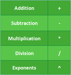
Illustration of mathematical operators
All formulas in Excel must begin with an equals sign (=). This is because the cell contains, or is equal to, the formula and the value it calculates.

Understanding cell references

While you can create simple formulas in Excel manually (for example, =2+2 or =5*5), most of the time you will use cell addresses to create a formula. This is known as making a cell reference. Using cell references will ensure that your formulas are always accurate because you can change the value of referenced cells without having to rewrite the formula.
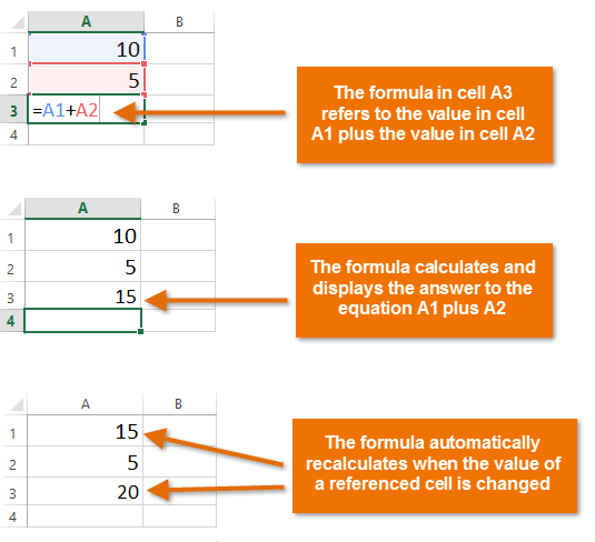
Screenshot of Excel 2013
By combining a mathematical operator with cell references, you can create a variety of simple formulas in Excel. Formulas can also include a combination of cell references and numbers, as in the examples below:
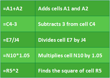
Illustration of simple formulas

To create a formula:

In our example below, we'll use a simple formula and cell references to calculate a budget.
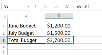
  1. Select the cell that will contain the formula. In our example, we'll select cell B3.
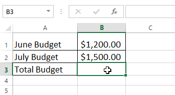
    Screenshot of Excel 2013
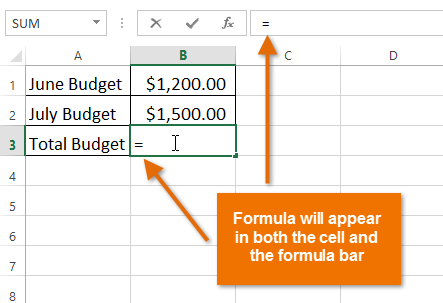
  2. Type the equals sign (=). Notice how it appears in both the cell and the formula bar.
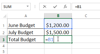
  3. Type the cell address of the cell you want to reference first in the formula: cell B1 in our example. A blue border will appear around the referenced cell.
    Screenshot of Excel 2013
  4. Type the mathematical operator you want to use. In our example, we'll type the addition sign (+).
  5. Type the cell address of the cell you want to reference second in the formula: cell B2 in our example. A red border will appear around the referenced cell.
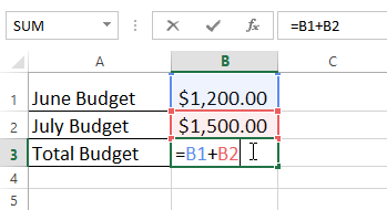
    Screenshot of Excel 2013
  6. Press Enter on your keyboard. The formula will be calculated, and the value will be displayed in the cell.
    Screenshot of Excel 2013
If the result of a formula is too large to be displayed in a cell, it may appear as pound signs (#######) instead of a value. This means the column is not wide enough to display the cell content. Simply increase the column width to show the cell content.

Modifying values with cell references

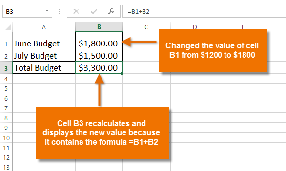
The true advantage of cell references is that they allow you to update data in your worksheet without having to rewrite formulas. In the example below, we've modified the value of cell B1 from $1,200 to $1,800. The formula in B3 will automatically recalculate and display the new value in cell B3.
Screenshot of Excel 2013
Excel will not always tell you if your formula contains an error, so it's up to you to check all of your formulas. To learn how to do this, you can read the Double-Check Your Formulas lesson from our Excel Formulas tutorial.

To create a formula using the point-and-click method:

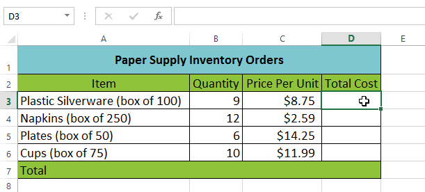
Rather than typing cell addresses manually, you can point and click on the cells you want to include in your formula. This method can save a lot of time and effort when creating formulas. In our example below, we'll create a formula to calculate the cost of ordering several boxes of plastic silverware.
  1. Select the cell that will contain the formula. In our example, we'll select cell D3.
    Screenshot of Excel 2013
  2. Type the equals sign (=).
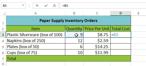
  3. Select the cell you want to reference first in the formula: cell B3 in our example. The cell address will appear in the formula, and a dashed blue line will appear around the referenced cell.
    Screenshot of Excel 2013
  4. Type the mathematical operator you want to use. In our example, we'll type the multiplication sign (*).
  5. Select the cell you want to reference second in the formula: cell C3 in our example. The cell address will appear in the formula, and a dashed red line will appear around the referenced cell.
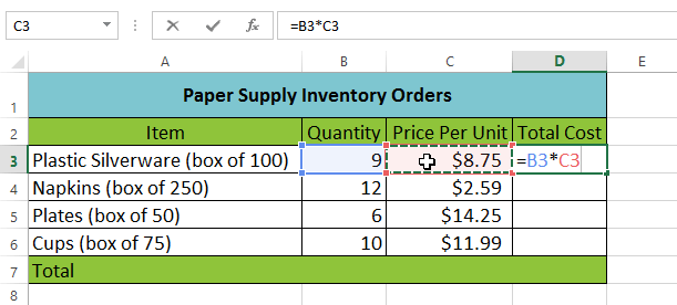
    Screenshot of Excel 2013
  6. Press Enter on your keyboard. The formula will be calculated, and the value will be displayed in the cell.
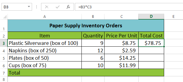
    Screenshot of Excel 2013
Formulas can also be copied to adjacent cells with the fill handle, which can save a lot of time and effort if you need to perform the same calculation multiple times in a worksheet. Review our lesson on Relative and Absolute Cell References to learn more.
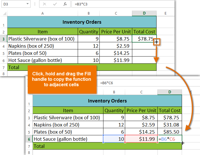
Screenshot of Excel 2013

To edit a formula:

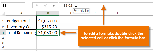
Sometimes you may want to modify an existing formula. In the example below, we've entered an incorrect cell address in our formula, so we'll need to correct it.
  1. Select the cell containing the formula you want to edit. In our example, we'll select cell B3.
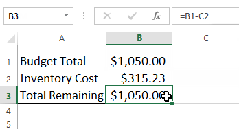
    Screenshot of Excel 2013
  2. Click the formula bar to edit the formula. You can also double-click the cell to view and edit the formula directly within the cell.
    Screenshot of Excel 2013
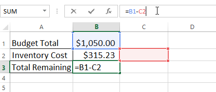
  3. border will appear around any referenced cells. In our example, we'll change the second part of the formula to reference cell B2 instead of cell C2.
    Screenshot of Excel 2013
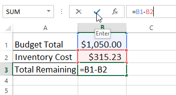
  4. When you're finished, press Enter on your keyboard or click the checkmark in the formula bar.
    Screenshot of Excel 2013
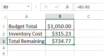
  5. The formula will be updated, and the new value will be displayed in the cell.
    Screenshot of Excel 2013
If you change your mind, you can press the Esc key on your keyboard to avoid accidentally making changes to your formula.
To show all of the formulas in a spreadsheet, you can hold the Ctrl key and press ` (grave accent). The grave accent key is usually located in the top-left corner of the keyboard. You can press Ctrl+` again to switch back to the normal view.

Current Affairs 31st January 2018 - Banking, SSC, UPSC Affairs

31st January Current Affairs 2018: Instantly obtain Latest Current Affairs 
January 31, 2018 with all essential info. Be the first to know all the 
Current affairs January 31, 2018 top news, Major Issues, 
Current happenings, Important events in National as well as 
International level with clear explanation. For all competitive exams 
and Interviews, equip yourself with the Latest Current Affairs 
January 31, 2018 granted here.


Axis Bank Launches fourth edition of Evolve

Private sector Axis Bank launched the fourth edition of ‘Evolve’ in Coimbatore, 
Tamil Nadu. It is an annual multi-city knowledge series for Bank’s small and 
medium-sized enterprises (SME) customers. The current edition of 'evolve' is 
titled as “Transform your Family Business into your dream company”. It will empower the 
SMEs to understand the winning strategies and best practices that have helped some of the leading 
family businesses in India grow into the reputable enterprise. This edition will span across 30 cities.

Google Introduces A New App Named as Bulletin

Google introduced a new app named "Bulletin" that allows anybody to submit 
stories for and about their communities. This is a free, lightweight app for 
telling a story by capturing photos, video clips and text right from your phone, 
published straight to the web. The app is made for contributing hyperlocal stories about your community. 
The application has been launched as a limited pilot project and is available in Nashville, Tennessee, 
and Oakland, California.

Melbourne To Host Final Of 2020 World T20

Melbourne Cricket Ground will host the final of both the men’s and women’s 
World Twenty20 when the tournaments come to Australia in 2020. It will mark
 the first time the tournaments are held as stand-alone events in the same year 
in the same country. The women’s final will coincide with International Women’s Day (8th March).


Prime Minister Narendra Modi Launched 1st Khelo India School Games

Prime Minister Narendra Modi launched the first Khelo India School Games at 
Indira Gandhi Indoor Stadium in New Delhi. The Khelo India programme has been
 introduced to revive the sports culture in India at the grass-root level. 
Talented Under-17 players identified in priority sports disciplines at various levels by a High-Powered 
Committee will be provided annual financial assistance of Rs. 5 lakh per annum for 8 years. 
The Khelo India School Games are being held from 31st January to 8th February 2018 in New Delhi.

Sharath Kamal Wins Table Tennis Nationals Championship

Sharath Kamal beat top-seeded Anthony Amalraj to win the men singles title for
 the eighth time, equalling the feat of Kamlesh Mehta in the 79th edition of the 
11Even Sports Senior Nationals in Ranchi, Jharkhand. Suthirta Mukherjee
 from West Bengal emerged the new women champion, beating Hyderabad Nationals winner Manika Batra.

India Ranks 6th In The List Of Wealthiest Countries

India ranked sixth in the list of wealthiest countries with the total wealth of 8,230
 billion US dollars. The list was topped by the United States of America, according to 
a report by New World Wealth. He was the best-performing wealth market 
globally in 2017 as its total wealth swelled from 6,584 billion dollars in 2016 to 8,230 billion dollars 
in 2017, registering a 25% growth.

Himachal Pradesh launches Zero Budget Natural Farming project to promote organic farming

Himachal Pradesh Government launched Zero Budget Natural Farming (ZBNF) project
 to promote organic farming. It was launched by Chief Minister, Jai Ram Thakur. 
The project aims to increase agriculture produce and the income of farmers by 
the year 2022. ZBNF is set of natural farming methods where the cost of growing and harvesting 
plants is zero. It is a farming practice that believes in the natural growth of crops without adding any 
fertilizers and pesticides or any other foreign elements.

Indian Navy launches third Scorpene class submarine Karanj

The Indian Navy launched ‘Karanj,’ the third Scorpene class submarine. 
The submarine, constructed by shipbuilder Mazagon Dock Limited (MDL) 
in Mumbai. The first of the six Scorpene-class submarines, Kalvari, 
was commissioned into the Indian Navy by Prime Minister Narendra Modi last month. 
He had called its induction a big step in the country’s defense preparedness. 
On the occasion, Defence Minister Nirmala Sitharaman had called submarine building a 
sophisticated and exacting craft, which only a handful of countries possess in their industrial capacity.

Environment Minister Harshvardhan Launches PetaFlop Super Computer

Environment Minister Harshvardhan launched a 2.8 PetaFlop capacity 
high-performance computer system ‘Mihir’ in Noida. The system will be 
able to predict weather and climate accurately. This will be helpful in 
addressing the various issues of agriculture operations and fishing in the country. The system 
will help the department in predicting severe climate-related calamities and warnings for fishermen.
 With the launch of the system, India has joined the elite 30 member group of countries which have
 this advanced technology.

Union Government Signs $250 Million Loan Agreement With ADB

The Asian Development Bank and the Indian Government signed a 250 million 
dollar loan to finance the construction of over 6 thousand 2 hundred kilometers
 all-weather rural roads in 5 states viz Assam, 
Chhattisgarh, Madhya Pradesh, Odisha and West Bengal under the Pradhan Mantri 
Gram Sadak Yojana (PMGSY). The program is aimed at improving rural connectivity, 
facilitating safer and more efficient access to livelihood and socio-economic 
opportunities for rural communities through improvements to about 12 thousand
 kilometers Rural Roads across the 5 States.

India to witness super blue moon with lunar eclipse

India would witness a 'super blue blood' moon between 5:15 PM and 7:37 PM on
 as the Moon goes from east to west. Occurring for the first time since 1866, 
the second Full Moon of the month, often called a Blue Moon, 
would coincide with a lunar eclipse giving it a blood-red tint, with the Moon also being a supermoon.

India becomes third largest producer of crude steel

According to a recent report published by World Steel Association (WSA), 
India overtook the US to become the world’s third-largest steel producer in 2018.
 China has remained world leader by producing 831.7 MT in 2017, 
up 5.7% from 786.9 MT in the year-ago period.   Japan is second largest global steel producer. 
The Global steel production had reached 1,691.2 MT in 2017, up by 5.3% compared to 2016 
when output was 1,606.3 MT. It includes over 160 steel producers with 9 of 
the 10 largest steel companies, national and regional steel industry associations, 
and steel research institutes. It was founded in July 1967 and is headquartered in Brussels, Belgium.

Indian-American Adobe CEO Shantanu Narayen To Lead USISPF Board

Indian-American Adobe CEO Shantanu Narayen elected as the Vice 
Chairman of the US-India Strategic and Partnership Forum. 
It is a new organization set up to enhance business 
relations between India and the US. The new representative body - 
US-India Strategic Partnership Forum (USISPF) was set up to promote bilateral trade
 and work on creating meaningful opportunities that have the power to change the lives of citizens. 
The USISPF now has 31 board members.


Tag: current affairs 2018,current affairs in india,current affairs quiz,current affairs 2017 pdf,current affairs in hindi pdf,
current affairs pdf,current affairs funda,current affairs,current affairs today,current affairs affairs cloud,
current affairs and gk,current affairs banking,current affairs bits,b.ed current affairs,b.sc current affairs

Tuesday, 30 January 2018

Getting Started with Excel

Introduction

Excel 2010
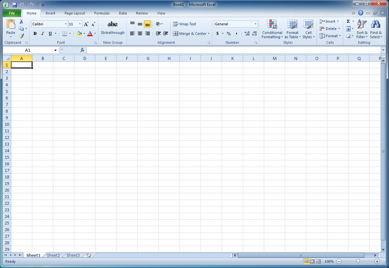
Excel is a spreadsheet program that allows you to store, organize, and analyze information. In this lesson, you will learn your way around the Excel 2010 environment, including the new Backstage view, which replaces the Microsoft Office button menu from Excel 2007.
We will show you how to use and modify the Ribbon and the Quick Access toolbar, as well as how to create new workbooks and open existing ones. After this lesson, you will be ready to get started on your first workbook.

Getting to know Excel 2010

Video: Navigating Excel 2010

Launch video!
The Excel 2010 interface is similar to Excel 2007. There have been some changes we'll review later in this lesson, but if you're new to Excel first take some time to learn how to navigate an Excel workbook.

The Excel interface

Click the buttons in the interactive below for an overview of how to navigate an Excel workbook.
labeled graphic

Working with your Excel environment

Video: Exploring Your Excel 2010 Environment

Launch video!
The Ribbon and Quick Access toolbar are where you'll find the commands you need to perform common tasks in Excel. If you are familiar with Excel 2007, you will find that the main difference in the Excel 2010 Ribbon is that commands such as Open and Print are now housed in Backstage view.

The Ribbon

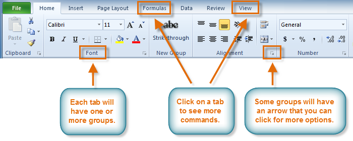
The Ribbon contains multiple tabs, each with several groups of commands. You can add your own tabs that contain your favorite commands.
Overview of the Ribbon
Certain programs—such as Adobe Acrobat Reader—may install additional tabs to the Ribbon. These tabs are called add-ins.

To customize the Ribbon:

You can customize the Ribbon by creating your own tabs that house your desired commands. Commands are always housed within a group, and you can create as many groups as you need to keep your tabs organized. You can also add commands to any of the default tabs as long as you create a custom group within the tab.
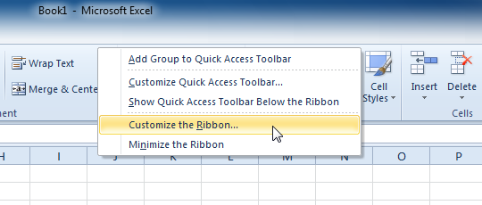
  1. Right-click the Ribbon, then select Customize the Ribbon. A dialog box will appear.
    Right-clicking the Ribbon to customize it
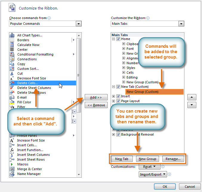
  2. Click New Tab. A new tab will be created with a new group inside it.
  3. Make sure the new group is selected.
  4. Select a command from the list on the left, then click Add. You can also drag commands directly into a group.
  5. When you are done adding commands, click OK.

    Customizing the Ribbon
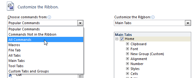
If you do not see the command you want, click the Choose commands drop-down box and select All Commands.
Displaying All Commands

To minimize and maximize the Ribbon:

The Ribbon is designed to be easy to use and responsive to your current tasks; however, if you find that it's taking up too much of your screen space, you can minimize it.
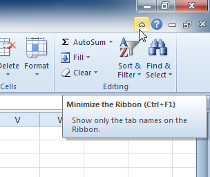
  1. Click the arrow in the upper-right corner of the Ribbon to minimize it.
    Overview of the Ribbon
  2. To maximize the Ribbon, click the arrow again.
When the Ribbon is minimized, you can make it reappear by clicking a tab. However, the Ribbon will disappear again when you're not using it.

The Quick Access toolbar

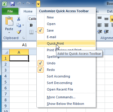
The Quick Access toolbar, above the Ribbon, lets you access common commands no matter which tab you are on. By default, it shows the SaveUndo, and Repeat commands. You can add other commands to make it more convenient for you.

To add commands to the Quick Access toolbar:

  1. Click the drop-down arrow to the right of the Quick Access toolbar.
  2. Select the command you want to add from the drop-down menu. To choose from more commands, select More Commands.
    Customize The Quick Access toolbar

Backstage view

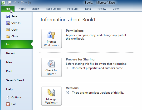
Backstage view gives you various options for saving, opening a file, printing, and sharing your document. It is similar to the Microsoft Office button menu from Excel 2007 and the File menu from earlier versions of Excel. However, instead of just a menu it's a full-page view, which makes it easier to work with.

To get to Backstage view:

  1. On the Ribbon, click the File tab.
    Backstage view
  2. Choose your desired option, or return to your workbook by clicking any tab on the Ribbon.
Click the buttons in the interactive below to learn about the different things you can do in Backstage view.
labeled graphic

Creating and opening workbooks

Video:Creating Workbooks in Excel 2010

Launch video!
Excel files are called workbooks. Each workbook holds one or more worksheets (also known as spreadsheets).

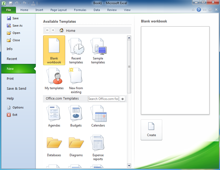
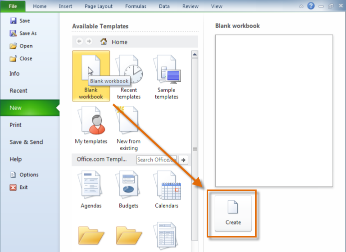
To create a new blank workbook:

  1. Click the File tab. This takes you to Backstage view.
  2. Select New.
  3. Select Blank workbook under Available Templates. It will be highlighted by default.
  4. Click Create. A new blank workbook appears in the Excel window.
    Creating a new workbook
To save time, you can create your document from a template, which you can select under Available Templates. We'll talk more about this in a later lesson.

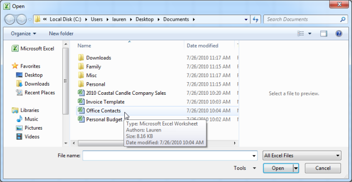
To open an existing workbook:

  1. Click the File tab. This takes you to Backstage view.
  2. Select Open. The Open dialog box appears.
    Opening a workbook
  3. Select your desired workbook, then click Open.
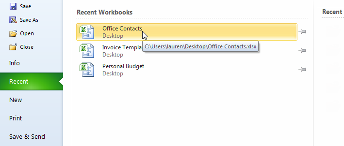
If you have opened the existing workbook recently, it may be easier to choose Recent from the File tab instead of Open to search for your workbook.
Opening a recent workbook

Compatibility mode

Sometimes you may need to work with workbooks that were created in earlier versions of Microsoft Excel, such as Excel 2003 or Excel 2000. When you open these types of workbooks, they will appear in Compatibility mode.
Compatibility mode disables certain features, so you'll only be able to access commands found in the program that was used to create the workbook. For example, if you open a workbook created in Excel 2003 you can only use tabs and commands found in Excel 2003.
In the image below, the workbook has opened in Compatibility mode. You can see that the sparklines and slicers features have been disabled.
Screenshot of Excel 2010
To exit Compatibility mode, you'll need to convert the workbook to the current version type. However, if you're collaborating with others who only have access to an earlier version of Excel, it's best to leave the workbook in Compatibility mode so the format will not change.

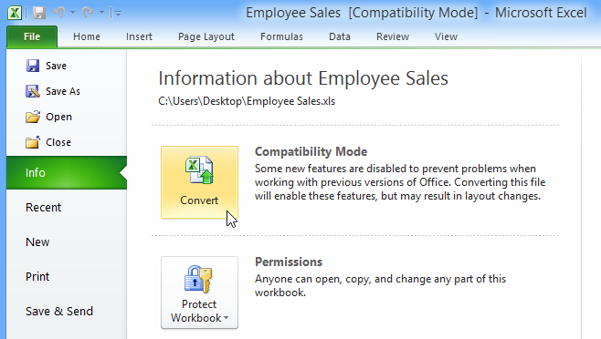
To convert a workbook:

If you want access to all of the Excel 2010 features, you can convert the workbook to the 2010 file format.
Note that converting a file may cause some changes to the original layout of the workbook.
  1. Click the File tab to access Backstage view.
  2. Locate and select the Convert command.
    Screenshot of Excel 2013
  3. The Save As dialog box will appear. Select the location where you want to save the workbook, enter a file name for the presentation, and click Save.

    Screenshot of Excel 2010
  4. The workbook will be converted to the newest file type.